Validating the state-basd elastic model (2D)
This example shows that the simulations recovers the discplacement predicted by classical continnums mechanics for a given load in force. The full example is shown in the following publication:
- Diehl, P., Jha, P.K., Kaiser, H. et al. An asynchronous and task-based implementation of peridynamics utilizing HPX—the C++ standard library for parallelism and concurrency. SN Appl. Sci. 2, 2144 (2020). https://doi.org/10.1007/s42452-020-03784-x.
Generating the mesh
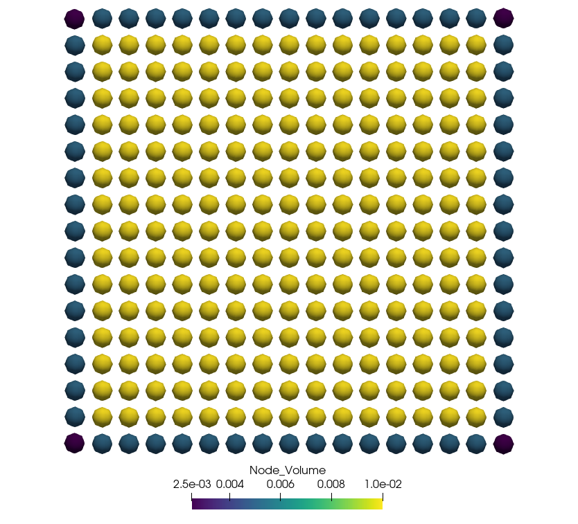
The file input_mesh.yaml in the example folder will generate the mesh as shown in the following figure.
Model
The quasi-static models as described in [1] is used to assemble the tangent stiffness matrix and obtain the solution by solving Newton steps.
Model:
  Dimension: 2
  Discretization_Type:
    Spatial: finite_difference
    Time: quasi_static
  Final_Time: 1
  Time_Steps: 1
  Horizon: 0.5
  Horizon_h_Ratio: 5
Material model
The state-based elastic material models as described in [2] is implemented for the ElasticState material.
Material:
  Type: ElasticState
  Density: 1200
  Compute_From_Classical: true
  K: 4000.0
  G: 1500.0
  Is_Plane_Strain: False
  Influence_Function:
    Type: 1
Applying boundary conditions
Displacement boundary conditions
The following code applies a fixed displacement to the first layer of nodes on the right-hand side in the first figure in both directions.
Displacement_BC:
  Sets: 2
  Set_1:
    Location:
      Line: [1.55, 1.65]
    Direction: [1]
    Time_Function:
      Type: constant
      Parameters:
        - 0.0
    Spatial_Function:
      Type: constant
  Set_2:
    Location:
      Line: [1.55, 1.65]
    Direction: [2]
    Time_Function:
      Type: constant
      Parameters:
        - 0.0
    Spatial_Function:
      Type: constant
Force boundary conditions
The following code applies a external body force density to the last node on the left-hand side in the first figure.
Note that in this example we want to apply a force $F=-40N$, however, the body force density has the units $\frac{N}{mm^2}$. Thus, the force is devided by the area $1.6\times 0.1$, where $1.6$ is the length of the plate and $0.1$ is the mesh width. This results in a body force density $-250$.
Force_BC:
  Sets: 1
  Set_1:
    Location:
      Line: [-0.1, 0.05]
    Direction: [1]
    Time_Function:
      Type: linear
      Parameters:
        - 1
    Spatial_Function:
      Type: constant
      Parameters:
        - -250.0
Solver
Solver:
  Type: BiCGSTAB
  Max_Iteration: 200
  Tolerance: 1e-6
  Perturbation: 1e-7
Validation
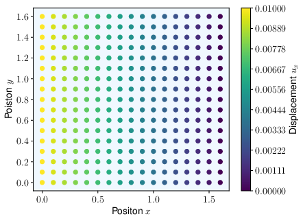
The prediction of the displacement field in $x$-direction is shown in second figure. For the derivation of the displacement field, we refer to [3].
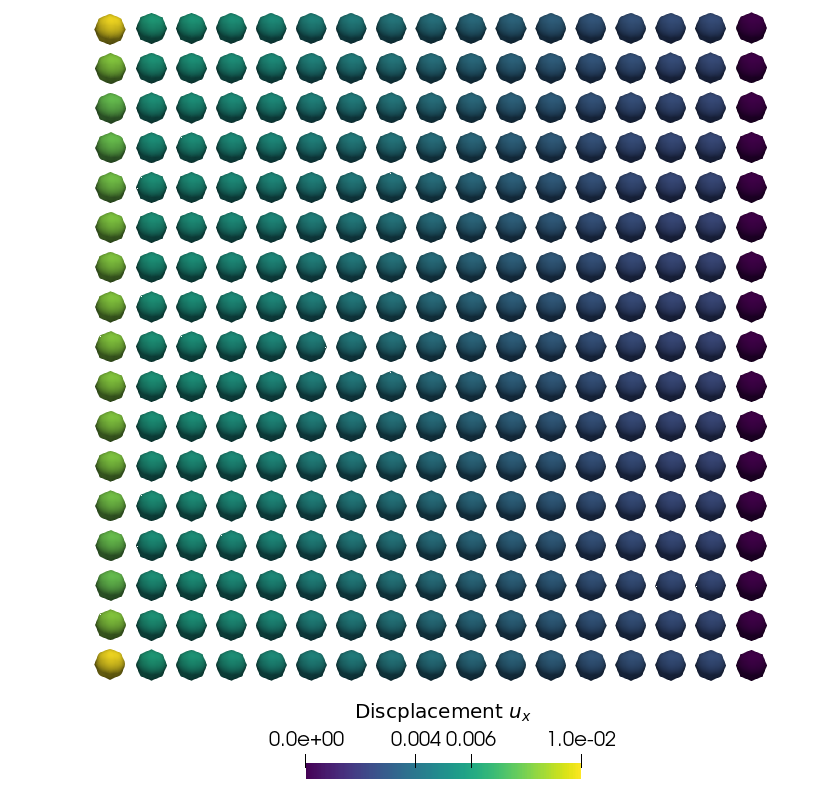
The third figure shows the obtained displacement field by the code using the above configuration.
References
- Littlewood, David J. “Roadmap for peridynamic software implementation.” SAND Report, Sandia National Laboratories, Albuquerque, NM and Livermore, CA (2015).
- Silling, Stewart A., et al. “Peridynamic states and constitutive modeling.” Journal of Elasticity 88.2 (2007): 151-184. 3.